R 語言:邏輯回歸 Logistic Regression using R language (二)
 > library('MASS')
 > data(menarche)
 > str(menarche)
 'data.frame':     25 obs. of 3 variables:
  $ Age   : num 9.21 10.21 10.58 10.83 11.08 ...
  $ Total  : num 376 200 93 120 90 88 105 111 100 93 ...
  $ Menarche: num 0 0 0 2 2 5 10 17 16 29 ...
 > summary(menarche)
    Age      Total      Menarche
  Min.  : 9.21  Min.  : 88.0  Min.  :  0.00
  1st Qu.:11.58  1st Qu.: 98.0  1st Qu.: 10.00
  Median :13.08  Median : 105.0  Median : 51.00
  Mean  :13.10  Mean  : 156.7  Mean  : 92.32
  3rd Qu.:14.58  3rd Qu.: 117.0  3rd Qu.: 92.00
  Max.  :17.58  Max.  :1049.0  Max.  :1049.00
上頭是 R 所提供的一個很好的 Logistic Regression with One numerical predictor 的例子。
簡單的說就是有一組三個自變數分別是 age, total 以及 menarche ,中文的大意是『我們收集了一共25組女性樣本,記錄每組的平均年紀,訪問次數以及受訪者是否發生初經』。
> plot(Menarch/Total ~ Age, data=menarche) 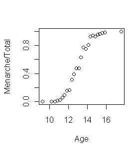
> glm.out = glm(cbind(Menarche, Total-Menarche) ~ Age, family = binomial(logit), data=menarche)
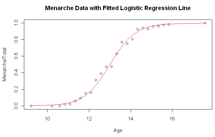
> plot(Menarche/Total ~ Age, data=menarche) + lines(menarche$Age, glm.out$fitted, col='red') + title(main='menarche data with fitted Logistic Regression Line')
 > summary(glm.out)
 Call:
 glm(formula = cbind(Menarche, Total - Menarche) ~ Age, family = binomial(logit),
   data = menarche)
 Deviance Residuals:
   Min    1Q  Median    3Q   Max
 -2.0363 -0.9953 -0.4900  0.7780  1.3675
 Coefficients:
        Estimate Std. Error z value Pr(>|z|)
 (Intercept) -21.22639  0.77068 -27.54  <2e-16 ***
 Age      1.63197  0.05895  27.68  <2e-16 ***
 ---
 Signif. codes: 0 '***' 0.001 '**' 0.01 '*' 0.05 '.' 0.1 ' ' 1
 (Dispersion parameter for binomial family taken to be 1)
   Null deviance: 3693.884 on 24 degrees of freedom
 Residual deviance:  26.703 on 23 degrees of freedom
 AIC: 114.76
 Number of Fisher Scoring iterations: 4
上圖的結果真是十分神奇,幾乎 match了!另外也可以確認這些結果: glm.out$coef, glm.out$fitted, glm.out$resid, glm.out$effects, and anova(glm.out). 另外文件上有提到,y 亦可視為是 odds, 所以可以解釋為每增加一歲, 即會增加 $\exp{1.63197} = 5.11$ 倍 "for every one year increase in age the odds of having reached menarche increase by 5.11 times".
 >1./(1+exp(-1*c(1,18)%*% glm.out$coef))
      [,1]
 [1,] 0.9997111
 > 1./(1+exp(-1*c(1,12)%*% glm.out$coef))
      [,1]
 [1,] 0.1620879
最後是關於這個 model 的評價。主要是看兩個部分:null deviance 與 residual deviance 。
null deviance 表示預測的結果有多好(越大越好), 這次預測是 chi-square value on 24 degrees of freedom, 表示 very little fit (a highly significant difference bw fitted values and observed values).= 在 1個自由度內降低 3667 points = a chi-square value 及 a high significant decrease in deviance.
residual deviance 則是誤差,這次預測 26.7 on 23 degrees of freedom, 我們利用此檢視是否發生 overfit (overall fit of the model). [這裏可透過 chi-square + df 計算 p-value]
"A chi-square of 26.7 on 23 degrees of freedom yields a p-value of 0.269. The null hypothesis (i.e., the model) is not rejected. The fitted values are not significantly different from the observed values"
個人的理解是:由於 residual deviance 的 p-value > 0.05, 表示 result isn't significant, 我們沒有信心推翻虛無假設($H_0$), 所以 fitted values 與 observed value 非 significant.
參考(1)

Comments
Post a Comment